Is it okay to rerandomise when running an experiment?
TL;DR - When running an experiment, sometimes we get unlucky and end up with imbalanced groups. Ensuring balance via rerandomisation can lead to more precise estimates. However, unless we account for this in standard error calculations, our inference will be invalid, and will infact lead to lower estimated precision.
Disclaimer: This post does not reflect the views of any employer.
All supporting code is available on github.
So you’re running an experiment, randomise your units into different conditions, and find that the units in one condition look pretty different to the units in other conditions. Bad luck, but what can you do about it? The answer is far from obvious and here I’ll demonstrate why.
The problem
Well-implemented randomisation ensures that on average, groups assigned different conditions will be similar. However, while this is true on average, in any one randomisation draw we may well have imbalances. When randomising across a population of individuals, we could end up with one group consisting of say, more men than another group. If in this example, being male is correlated with the outcome variable, intuitively its going to be harder to separate out the ‘effect’ (not necessarily causal) of being male from the effect of being in one experimental condition.
This type of imbalance becomes less likely as the number of units gets larger. However we may still worry even in large samples because:
- We don’t always randomise at the finest unit possible. For example, you may choose to randomise at the region level rather than the person level. This can radically reduce the effective sample size.
- As the sample size gets larger, estimates become more precise and hence small differences between groups have more of an impact.
What can we do in those circumstances? Can we just throw out that unlucky draw and re-randomise until we obtain balanced groups? Is that statistically valid?
This is addressed in a paper by Morgan and Rubin, published in 2012 in the Annals of Statistics. The paper itself is thorough and contains full statistical explanation, building on a wide body of earlier work. Here I’ll try to synthesise the paper’s practical implications, demonstrating the paper’s core points via simulation.
Rerandomisation can lead to greater precision
Getting an unlucky draw doesn’t bias your estimated treatment effect. Provided the standard conditions hold (e.g. SUTVA) your estimate will still be unbiased. This means that if you were to replicate the experiment over and over you would get the right answer. However, your estimated treatment effect may well be noisy, in that any one single estimate could be far from the truth.
Intuitively, rerandomisation should reduce the level of random noise, allowing us to obtain more precise estimates. In the supporting notebook, I set up a simulation to test this. I simulate some data on an outcome variable and ten covariates which are predictive of the outcome. I then simulate 1,000 experiments with two conditions, and for each draw calculate the following estimates:
- A ‘baseline’ treatment effect estimate based on a single randomisation.
- A ‘rerandomised’ treatment effect estimate in which I rerandomise until the treated and control groups are similar in terms of covariate means.
To assess ‘similarity’ here, we need a measure of distance. I use Euclidian distance, which is proportional to the sum of squared deviations between covariate means. I determine balance to be sufficient if this distance measure falls below some tolerance level.
The true simulated treatment effect is 1 unit. The figure below plots the treatment effect estimates for the 1,000 simulations.
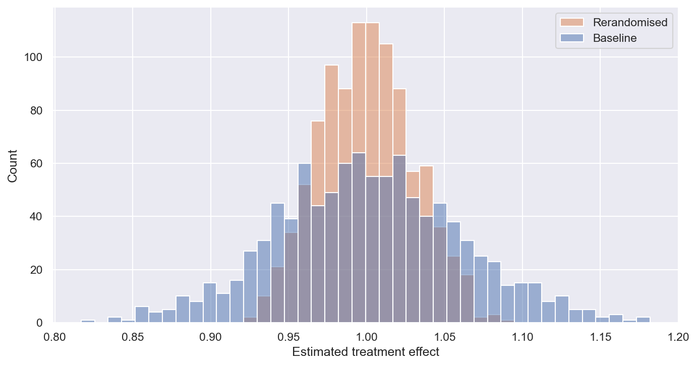
This shows:
- Both methods are unbiased, as they are centred at the true effect (1).
- The ‘rerandomised’ version is more precise, meaning that the variance of the estimates is lower. On average, the estimates are closer to the true effect (1).
Naive standard error estimates move the wrong way
The above evidence looks pretty good for rerandomisation. However, things get more complicated when we look at inference, i.e. how we estimate the uncertainty of our treatment effect estimates. First, let’s look at the estimated standard errors:
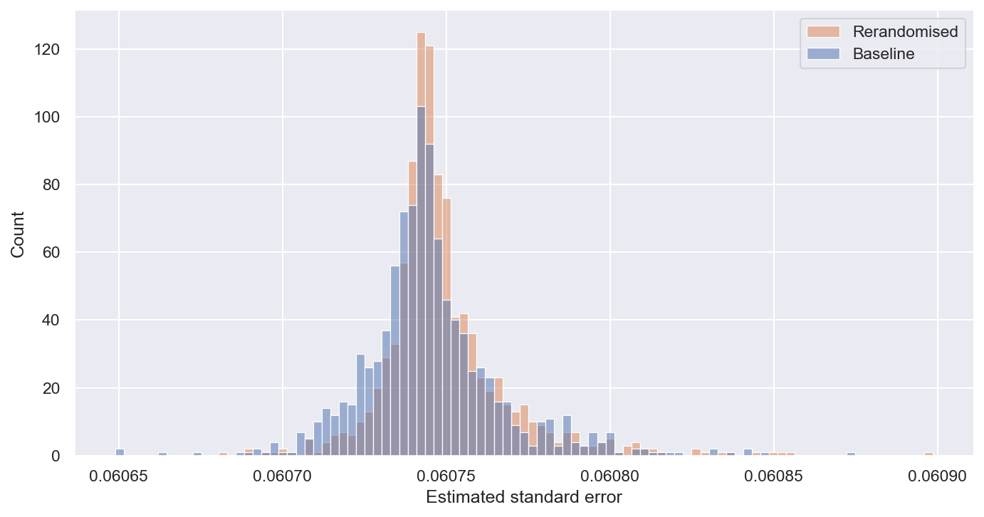
Above, we observed that true standard errors of treatment effect estimates are lower under rerandomisation, but here we see that estimated standard errors are actually marginally (0.7%) higher under rerandomisation. Why is this?
The typical way of estimating standard errors in randomised experiments is to use Neyman’s variance estimator. This uses the within-group variance to estimate the variance of the treatment effect estimate. When we balance our treatment and control group assignment via rerandomisation, we are reducing the cross-group variance. A knock-on effect of this is that we increase the within-group variance.
Inference based on naive standard errors is invalid
What does the above mean for our inference? A good way to see this is to look at the distribution of t-values under the null hypothesis of no treatment effect.
We can do this again via an identical simulation exercise, but this time we won’t add on any treatment effect. Given the true treatment effect is zero, for our inference approach to be valid, t-values should approximately follow a standard normal distribution. Our p-values and confidence intervals are based on this distribution. Systematic deviations suggest any inference we make based on these estimates are invalid.
In the below figure I plot the distribution of t-values for the baseline (no rerandomisation) and the rerandomisation alternative against a standard normal distribution.
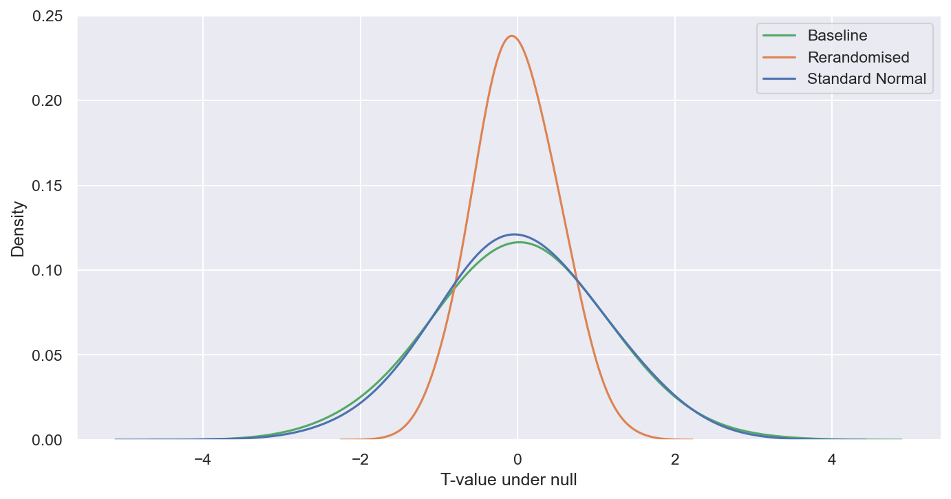
The baseline is well-aligned with the standard normal, as we would expect given the plain vanilla setup. However, the rerandomised t-values exhibit lower variance than the standard normal. This is because the standard error estimates are not reflecting the increased precision obtained via rerandomisation. In fact, as shown above they are going in the opposite direction.
If we rerandomise without adjusting standard errors, we will end up with overly conservative p-values and confidence intervals, leading us to under-reject the null hypothesis.
Summing up
Rerandomisation can increase precision, but without some adjustment of standard error calculations we will end up with invalid inference.
In their paper, Morgan and Rubin set out a strategy for adjusting standard errors to reflect the rerandomisation process under certain conditions, resulting in potentially higher precision while retaining valid inference. The process is sufficiently dense to be left for a later post.
In most cases, a point estimate isn’t enough and we need a sense of statistical significance before making a decision. If rerandomising without making any inference adjustments, you should be aware that your inference is going to be overly conservative, and hence you won’t be able to fully exploit the benefits of the approach.
As a practical point, the above only refers to erandomisation based on covariate imbalance. Rerandomising because a particular unit falls into a particular condition is a recipe for disaster, and can result in biased treatment effect estimates.